
Hey ya’ll. Hope your summer is going well! In the season of peaches and watermelon, it’s easy to take things for granted. No one has experienced this more than the optimization algorithms used in, well, just about every single machine learning and computational problem.
I thought, for this post, I would dive into one of the classics: the Broyden Fletcher Goldfarb Shanno algorithm, also known as BFGS, named after these ballers right here.

Before I get into the details of BFGS, I’m going to go into a little bit of the background of gradient based optimization.
A Brief Story:
Imagine you and two friends are blindfolded on a hill, and ya’ll want to find the lowest point: winner get a burrito and mangos. One of your friends, let’s call him Kuzko, decides to randomly hop around until he finds the lowest point. Kuzko will be hopping for a while.
Your other friend, let’s call him Tschaikowsky, is a little smarter. He decides to use some of the information he has, which is his current position. He can feel the slope of the ground by estimating the difference in heights beneath his two feet, and uses that to choose his direction. He’s going to be pretty darn tough to beat.
There is a flaw in Tschaikowsky’s approach: to avoid ever going uphill, he avoids taking big steps. So you realize that, if you can figure out both what direction to go, and how far to go in that direction, you will be victorious. Because you have a deep grasp of physical geometry, you are able to estimate from your position not only the slope of the hill, but also how fast the hill is changing. This takes you a little extra time, and you end up taking fewer steps than Tschaikowsky and way fewer than Kuzko, but because each of you steps are much more informed than either of your friends, you find the minimum the fasted and have won the burrito!

Into the Math:
Optimization is exactly what you just did: trying to find the lowest point on an N-dimensional hill while being blindfolded. Just like your game, there are many different methods to find the local minimum. But with each dimension you add, the more important your method’s precision or efficiency becomes.
However, since an optimizer does not possess feet, the mathematical equivalent of estimating the hill-space is the Taylor Series, which is defined as:
![]()
for small ![]()
It looks a little scary, but it’s really no different than the hill problem. The first term ![]() is simply the equivalent to your position on the hill. The second term,
is simply the equivalent to your position on the hill. The second term, ![]() is just the slope of the optimization space, or in our case, the hill. The final term is a measure of the change in the hill’s slope in each direction, also known as the Hessian matrix. The only difference between this equation and our little game is that you can apply this equation to an infinite number of dimensions.
is just the slope of the optimization space, or in our case, the hill. The final term is a measure of the change in the hill’s slope in each direction, also known as the Hessian matrix. The only difference between this equation and our little game is that you can apply this equation to an infinite number of dimensions.
We are looking for the optimal step to take, or the optimal ![]() , which can be found by taking the derivative in respect to delta X:
, which can be found by taking the derivative in respect to delta X:
![]()
From there, we solve for delta X to find
![]()
First Order Optimization:
It turns out your friend Tschaikowsky was pretty bright. An entire class of optimizers, called first order optimizers, actually only use the gradient and ignore the Hessian. however, for reasons of computational efficiency as well as other more nuanced reasons (a topic for another post), only use the gradient and not the hessian (2nd order gradient) to optimize a loss function. Thus, first order gradients approximate this approximate this approximation by simply setting
![]()
These first order algorithms are known as SGD, Adam, Adadelt optimizers typically used in deep learning frameworks such as Tensorflow and PyTorch. However, just like Tchaikovsky, this method has the flaw that it contains no information of what size step to take. The danger in this is that if the gradient is large, i.e. the hill has a large slope, but the slope is rapidly decreasing, the gradient would still tell you to take a giant step.
However, because the Hessian grows at a factor of ![]() , the “solution” to this issue is to simply set
, the “solution” to this issue is to simply set ![]() to a very small value so that the Hessian terms become in consequentially small.
to a very small value so that the Hessian terms become in consequentially small.
Take the plot below for example, which depicts a first order optimizer with a step size of 1 and step-size 0.1
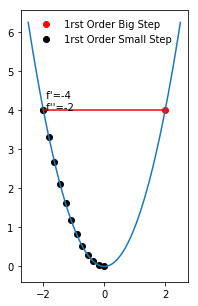
As you can see, even optimizing a simple parabola, with too large a step size, the gradient will never converge, bouncing around near the local minimum. The alternative is optimizing the parabola with a small step size, which eventually finds the local minimum, but is very inefficient about the number of iterations it takes.
Second Order Optimization:
However, by including the Hessian matrix in the optimization, the step size is automatically scaled in respect to the optimization space. However, now we also have to calculate the Hessian matrix at each step.
The major drawback with this method is, for a long time, calculating the Hessian matrix was such an expensive computation that the benefit of an adaptive step/direction scaling simply wasn’t worth it. Until our boys BFGS came along and developed an extremely efficient way to approximate the inverse Hessian matrix ( Disclaimer- I personally believe Davidson-Fletcher-Powell deserve a lot more credit, as the solved the problem of approximating the Hessian matrix: BFGS literally took their formula and applied it instead to the inverse Hessian. But history is written by the winners, and BFGS turned out to work slightly better).
The BFGS algorithm is in the family of Quasi-Newton which is a family of optimization methods BFGS algorithm does this through continuously updating the Hessian matrix based on information from the current change in gradient, the current step, and the previous Hessian. The assumption of this algorithm is that there is enough information in the gradient at ![]() and
and ![]() , as well as the Hessian
, as well as the Hessian ![]() to estimate the
to estimate the ![]()
![]()
The approach BFGS took is to use this easy to compute information to build two estimates of ![]() , that provide complementary information. Let’s call them
, that provide complementary information. Let’s call them ![]() and
and ![]() .
.
One way to develop a reasonable estimate of the Hessian matrix is to simply take the matrix multiplication of the change in gradient vector, s.t.
![]()
Where
![]()
This is essentially a first order estimate of the Hessian matrix, and is a measure of how much the gradient of each direction changed in respect to every other direction between position A and position B. However, the reason we want to compute the Hessian matrix is to avoid relying on first order estimates, so this estimate alone would not bring too much new information. So that brings in the second order estimate of the Hessian matrix:
![]()
Where ![]() is an estimate of
is an estimate of ![]() based on the previous Hessian matrix
based on the previous Hessian matrix
The new Hessian ![]() can then be estimated by:
can then be estimated by:
![]()
Where
![]()
![]()
If this form looks a little familiar, it should. We have are estimating a new term ![]() based on the previous term
based on the previous term ![]() , a scaled first order estimate of the
, a scaled first order estimate of the ![]() value and a scaled second order estimate of the
value and a scaled second order estimate of the ![]() value. This is exactly the same form as our estimate of
value. This is exactly the same form as our estimate of. Think about that beautiful symmetry: we are using a formula that almost mirrors a Taylor series expansion to approximate the Hessian
![]() so that we can use the Hessian in our Taylor series approximation of
so that we can use the Hessian in our Taylor series approximation of .
My goal in this write-up was to give an overview of optimization methods, the difference between first and second order optimization, and in-depth study towards the motivations and effect of the BFGS algorithm. I didn’t dive too heavily into the proof of the BFGS algorithms, simply because the proof is about 4-5 pages of algebra, and instead chose to focus more on the intuition which I believe is more valuable. However, if you are interested, there is a great set of lecture slides that dives into a full derivation of the DFP and BFGS methods.
That’s all for now- hope you enjoyed!