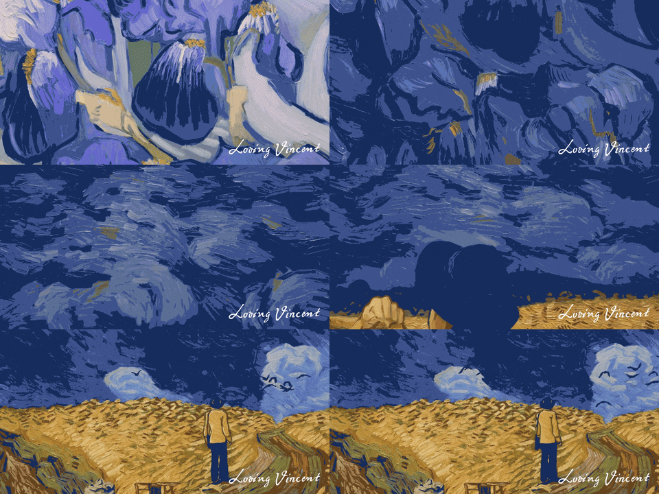
A few days ago, I watched this movie called Loving Vincent, and the visual beauty of the movie blew me away.

259 artists over a five year stretch painted every single frame of the film. This was a project of passion and the passion brought Van Gogh’s paintings to life, each second a visual heartbeat for the film.
But this isn’t a movie review blog. I do numbers. Of course, there’s no replacement for the passion and artistry that it took to create a work of art like Loving Vincent. However, I did want to see there were a way to better bring paintings and artwork to life mathematically.
I’m sure someone smarter than me could think of a way to set this up as a deep learning problem, design some kind of deep CNN, and find some sort of proxy metric to optimize to find filters that perturb images in an interesting way.
But I don’t really feel like doing that. And I also don’t think that such a black-box based method is the move, especially when using ambiguous objectives such as “coolness” or “aliveness.” Instead, I decided to hand-craft pixel-wise perturbation matrix to bring images to life.
Method 1: Multiplication Matrix
The first method I tried was a pixel-wise multiplication operation. I build a matrix with each value drawn from a normal distribution centered at 1 with a standard deviation of 0.3. We use Van Gogh’s Starry Night to test the image because beatifulness.
Code for Method 1

delta = np.random.normal(loc=1, scale=.03, size=myimg.shape[0:2])
delta = np.expand_dims(delta, -1)
dimg = np.multiply(myimg, delta)
myimg = dimg
I run this algorithm to perturb the image 45 times to get 45 new perturbed images. I also save each delta matrix and run the pointwise division to get 45 more images. The 90th image is the same as the first. I compile these images to create a video. Check it out below.
This looks a little interesting. There is some interesting twinkling. But very few regions of the paintings appear to be affected. Specifically, only the stars appear to undergo any perturbation.
Lighter colors have higher RGB values. Multiplication will scale larger values more than it will scale smaller values: thus bright colors will consistently be more affected than smaller colors. This is not neccessarily a bad thing, but it looks bad, and seeing as coolness is our metric, we now know what to change.
Method 2: Addition Matrix
Instead of running pointwise multiplication, we can run pointwise addition. We will use the same value to scale each R, G, and B value in order to keep colors reasonably consistent. We draw our values from a normal distribution centered around 0 with a standard deviation of 2.
Code for Method 2

    delta = np.random.normal(loc=0, scale=2, size=myimg.shape[0:2])
    delta = np.expand_dims(delta, -1)
    dimg = myimg + delta
    myimg = dimg
However, this method seems to barely do anything to the image. I realize the reason for this is because the normal distribution is centered at 0. Thus, in the average case, a pixel value will change by 0. This is bad: let’s change it.
Method 3: Shifted Addition
Very similar to method 3. However, we instead center the normal distribution at 3 with a standard deviation of 1.5. Thus, in the average case, the pixel values will all consistently increase, and thus change.
Code for Method 3

    delta = np.random.normal(loc=3, scale=1, size=myimg.shape[0:2])
    delta = np.expand_dims(delta, -1)
    dimg = myimg + delta
    myimg = dimg
Now this one looks pretty dope. From here, we are just optimizing a working product. One thing that occurs as a result of centering our normal distribution at 3 is that all our delta values will be positive. In an image, that means our pixels will only grow brighter, which limits our space of coolness.
Darker transformations can be just as dope as brighter transformations. We can fix this issue by adding a simple random choice to multiply our values by 1 or negative 1.
Method 4: Random Mu for Normal
Now our image looks like it has a heartbeat. However, one potentialarea of improvement could be the fact that our transformations lack variety. Because we draw from the same normal distribution, over enough iterations, each transformation should look reasonably similar.
We can improve our variaty by adding a layer of randomization to our matrix. Instead of drawing our values from a set normal distribution, we can draw our normal distribution parameters from another distribution. I choose uniform.
Code for Method 4

    med = np.random.uniform(low=1, high=high)
    delta = sign*np.random.normal(loc=med, scale=med/2,
                                  size=myimg.shape[0:2])
    delta = np.expand_dims(delta, -1)
    dimg = myimg + delta
    myimg = dimg
This adds a layer of randomization and really makes our video come alive. There are definitely more levels of perturbation and changes we can add, but I’m very happy with this general frame work.
This also generalizes very well to other paintings as well. I posted some other paintings on the youtube:
So yeah. I just thought this was really sick. I thought it was a cool project and it shows how much you can do with pretty simple mathematical operations and following trial and error and intuition. And I think it makes art look really cool and gives it a sort of artistic heartbeat. I’ll see if I can deploy this at some point or you can just run the notebook/python script with any image that you want.
I posted my notebooks on github: https://github.com/ghodouss/ArtAlive
🙂
