What did the physicist say after the short, redhead spit on his shoe?
…
“Let me atom”

So with that subtle segway, let’s dive into our topic today: atomic physics and the reason why Markov Chain Monte Carlo is an effective method to estimate probabilities or a “Posterior distribution” given a loss function.
Think about the scale of atoms: they’re pretty small. In a single block of ice (in scientific terms, an ice crystal), there are about ![]() molecules of water. Yet, every time you freeze water, water molecules end up in the same atomic, crystalline shape. Imaging trying to get 1 million balls to line up in a perfectly straight line. Except that the balls just keep randomly moving as soon as you let them go. And now do that 1 million times and you’ll only have to organize 1 trillion more balls before you build the equivalent of an ice cube. Yet, below 0 degrees celsius, liquid water crystalizes almost instantaneously. That’s astounding!
molecules of water. Yet, every time you freeze water, water molecules end up in the same atomic, crystalline shape. Imaging trying to get 1 million balls to line up in a perfectly straight line. Except that the balls just keep randomly moving as soon as you let them go. And now do that 1 million times and you’ll only have to organize 1 trillion more balls before you build the equivalent of an ice cube. Yet, below 0 degrees celsius, liquid water crystalizes almost instantaneously. That’s astounding!

At the molecular level, there are a number of forces interacting: attractive and repulsive forces between atomic charges, hydrogen bonds, van der waals forces, etc. Without getting into the weeds, the point is that the various attractive and repulsive forces at play between the trillions and trillions of molecules create an extremely unstable and complex optimization space, far more complex than even the deepest of neural networks, because the free parameters are the positions of each atom. And that’s a lot of free parameters.
Yet, somehow, water is able to find the global minimum of this optimization space almost instantaneously. We know this because the structure of ice is a constant crystalline shape. The question, however, is how?
Detailed Balance:
Well, the answer is kind of a let-down: atoms are just really freaking fast. They are literally going through random perturbations until they reach the global optimal set of positions, broken down into local clusters. While this is a little discouraging, an entire field of optimization and sampling algorithms has emerged from mirroring the stochasticity of atoms while performing efficient probabilistic optimizations.
The primary key to keeping a sampling algorithm effectively equivalent to atomic optimization is this idea of detailed balance, which a metric that defines probabilistic purity. The key defining characteristic of detailed balance is, from the set of all transitions, a transition from point A to B must be as likely as a transition from point B to point A.
Now let me pause for a moment, and clarify (the statement above was difficult for me to wrap my head around at first). Let me put it into probabilistic terms:
Misconception:
![]()
True Equation:
![]()
The Difference:
The first equation states that the probability of transitioning from a point B to a point A is equal to the probability of transitioning from a point A to a point B. However, this implies that every point has the exact same probability. And that’s a pretty boring loss function.
The second equation states that the probability of transitioning from A to B and the probability of being at point B is equal to the probability of transitioning from point B to A and being at point A.
To make sense of this, think about a flipping a coin, where A is heads and B is tails. It’s a weighted coin, so ![]() and
and ![]() . So you would expect, after a large number of flips, the results to be about 70% A and 30% B. And in this case of absolute randomness,
. So you would expect, after a large number of flips, the results to be about 70% A and 30% B. And in this case of absolute randomness, ![]() and
and ![]() . Thus, in the case of absolute randomness,
. Thus, in the case of absolute randomness, ![]() . Thus, we change our sampling method to make it more efficient and still consider it a random sampling as long as our algorithm maintains detailed balance.
. Thus, we change our sampling method to make it more efficient and still consider it a random sampling as long as our algorithm maintains detailed balance.
The Metropolis Hastings Algorithm:
A very popular Markov Chain Monte Carlo algorithm, Metropolis Hastings defines a method to get a posterior distribution (random probabilistic sampling) much more efficiently than the atomic method of random perturbations. The algorithm has 3 Steps:
- Given the current position
 , use a perturbation function (e.g. a number selected from a normal distribution) to select a temporary position
- Calculate the ratio of the probabilities:
![]()
3. Set Next Position:
![]() with probability
with probability ![]() ,
,
Else ![]()
Detailed Balance in Metropolis Hastings
Let’s be a little more specific and describe some probabilities. The probability that you get ![]() from your perturbation function is:
from your perturbation function is:
![]()
where q is the probability of ![]() given your perturb function.
given your perturb function.
Let’s say you have point A and point B, and ![]() Then we need to find two values
Then we need to find two values
![]()
![]()
Thus we find that:
![]()
Well, dang. Go to the riverbed and call a tree Sally if that ain’t random!
Demonstration:
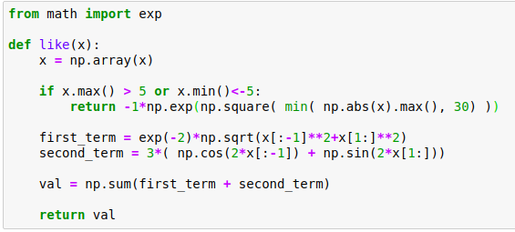
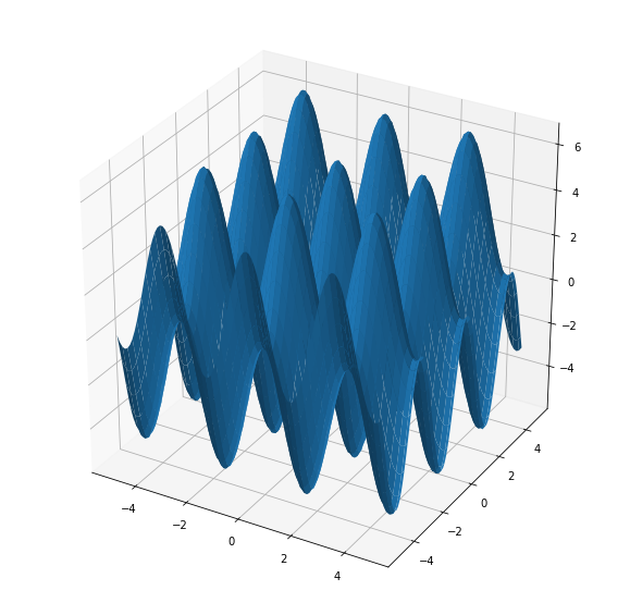
But, let’s go through an example Over the summer, part of my work was in the field of non-convex optimization. And in the process, I ran into some pretty darn nasty benchmark functions to optimize. One of them was the Acklay Function, which is defined as:
![]()
Or in other terms: Yuuuukkk!!!
 Now that we have a likelihood function, we are going to run an MCMC sampling algorithm to try to to get a representation of the Acklay function space. So to do this, I’m going to use a python library called emcee, which is a super light-weight library for probabilistic sampling. Emcee also uses a super useful optimization tool called affine invariant, which is a topic for another time. So first, I’m going to define our Acklay likelihood function:
I limit the range to between 5 and -5, which is to just limit computational expenses. Outside the range of (-5, 5), the likelihood exponentially decreases. From there, I use emcee to run a sampling of the likelihood space, and plot the histograms. I run samples from
And here are our approximations: 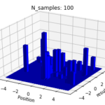
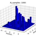
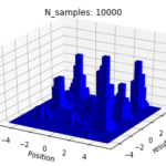
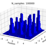
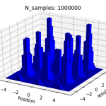
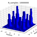
So you can see, with a probabilistic MCMC sampling, we are able to get an effective view of the entire optimization landscape of the loss function beyond a single point. We use a histogram, because the frequency at which a walker lands on a point should reflect the likelihood of that point, over a large number of iteration.
Hope ya’ll found this interesting! The parallels between atomic interactions and probabilistic sampling is a topic I just find fascinating and found worth sharing. Hope ya’ll enjoyed! |