No fun backstory for this post. These things are just cool and important in machine learning. Turns out they are very algorithmically similar. So I’ll explain how 🙂
Residual Blocks Review:
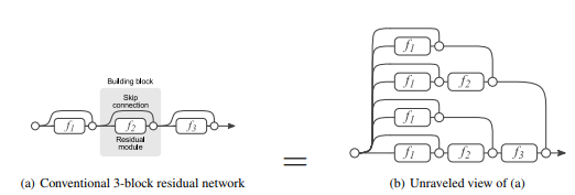
A residual block in a neural network is defined by the presence of skip layers, as seen in the id(Hk-1) connection in figure (1). These skip layers represent the addition of a layer i-k so some layer i . These blocks reduce the effect of vanishing gradients, and enable the development of much deep neural networks. This architecture enabled Microsoft to win the 2015 ImageNet challenge, and residual blocks have become a staple of deep neural networks.

Gradient Boosting Review:
Gradient boosting is a method for training an ensemble model of weak learners. I’ll unpack that statement.
Weak Learner
A weak model that, one its own, would struggle to fit the data, much less over fit. The most commonly used weak learners are decision trees with extremely early stopping, i.e. after 2-4 splits.
Classic Ensembles:
The idea behind ensembles is that by training models with some form of variation in them ( this variation can come in the form of the sub-sampling used by Random Forest Models or simply by training multiple models over a non-convex space through Monte Carlo Markov Chain sampling or Deep Learning models). The benefit of this sampling is an increase in generalizability beyond the training set. In a classic ensemble model, each individual model is trained with the objective of minimizing separate loss functions, and are ensembled at prediction time. The objective function of each model is:
![]()
Gradient Boosting:
Models within gradient boosted ensembles are not trained to optimize their own objective function but rather the ensemble’s objective function. The models in the ensemble are trained one at a time through gradient-based methods. However, unlike a normal gradient based machine learning model, the objective function:
![]()
Where ![]() is the current ensemble model and
is the current ensemble model and ![]() is the weak learner that is currently being trained. Thus, when running the gradient on the i+1 Model, the objective is not to minimize the loss for that model, but rather for the ensemble as a whole. This gradient boosting directly optimizes models for their prediction-time use case.
is the weak learner that is currently being trained. Thus, when running the gradient on the i+1 Model, the objective is not to minimize the loss for that model, but rather for the ensemble as a whole. This gradient boosting directly optimizes models for their prediction-time use case.
Same Old Song and Dance:
Let’s think about what each of these functions is really doing.
Layer i in the ResNet is defined as:
![]()
The Ensemble added with the ith model is defined as:
![]()
There are some differences, foremost among them being:
- The input to each ResNet Layer is dependent on the previous layer
- Each layer in the ResNet is trained simultaneously while earlier “layers” (models) in Gradient Boosting remain constant once trained.
However, within their respective domains of ensemble models and deep learning, gradient boosting and residual layers are doing very similar things. In a recent paper out of Cornell, it was demonstrated that skip-layers were effectively creating ensemble models. They demonstrated that, due to the nature of linear combinations, each separate path to the final output effectively represented a unique ensemble model.

They do a lot of cool stuff in this paper demonstrating this result, and I don’t want to steal their thunder, so I’ll just direct ya’ll straight to the source.
So What?
Well, it’s cool. I think that’s enough. But I did also have a hypothesis.
The major algorithmic difference between gradient boosting and ResNets is that previously trained models in the ensemble remain constant, while in the Resnet, they continually change. It may be interesting to see how well a deep neural network performs when trained 1 residual block at time. This method could drastically cut down on training time and drastically reduce the parameter space of the network.
Unfortunately, I do not an ensemble of GPUs at my disposal (“ensemble”- see what I did there?), but if anyone from Microsoft or Google or just some evil genius with 500 GPUs to spare is reading this, feel free to try it out.
